Can a search feel where it’s going?
A lightning strike begins from two directions. I’m investigating what that could teach us about a search finding its way.
Explore the ideaAn analogy. A small, solvable world.
A growing record of tests and questions.
The question behind the work
The next step is easy.
The right ending isn’t.
An answer grows one choice at a time. But a choice that looks good now can still lead somewhere wrong.
I’m exploring what happens when two things guide that process: an estimate of where a path will end, and a memory of paths taken before. Lightning offered the starting picture. Small, exactly solvable graphs gave me somewhere to test it.
In a typical negative cloud-to-ground flash, the connection grows from two directions. In the last moments before it connects, something rises to meet the descending leader: a short, faint discharge climbing from a rooftop, a mast, a tree, reaching up toward the channel coming down. The strike is the instant they touch. The bright bolt you actually see happens afterwards, running back up the path the two of them made together.
The upward half gave me the starting picture: a destination helps shape a route before the route is complete. Calling that “information from the destination” is an analogy. The physical process is electrical breakdown; the research question is whether a comparable mathematical structure can help explain a search.
A system that writes an answer one step at a time can already receive a goal in its prompt. What it generally lacks is the exact chance that each next choice will eventually reach that goal. I wanted to study what happens when a search is given that information, when the information is imperfect, and when its earlier choices leave a memory.
What follows is the record so far. A headline had to be demoted, an instrument turned out to be blind, and a prediction failed in exactly the place the idea was most attractive. The investigation continues through these loops: ask a question, test an idea, inspect the evidence, then decide what to ask next.
01
An intuition you can explore
Give the search
a sense of direction.
The world stays the same.
Change what the search knows.
One graph. Two directions.
An answer is a path.
Begin at one dot. Choose a line, arrive at another dot, choose again. Five steps lead to one of eight endings. Only one ending is the goal.
Every line is a possible next choice. The selected state and its next choices are lit. Brightness is lifted to keep faint paths visible; exact values are in the inspector.
There are 3 possible next choices from here.
| Next state | Ordinary chance |
|---|---|
| 35.47% | |
| 18.69% | |
| 45.84% |
The four readings, in words
An answer is a path.
Begin at one dot. Choose a line, arrive at another dot, choose again. Five steps lead to one of eight endings. Only one ending is the goal.
41 possible states. One start. Five more layers of eight.
The likeliest ending is wrong.
Give every choice its ordinary probability and let those probabilities flow forwards. The goal receives about one walk in eighty. The brightest ending is the decoy.
1.26% arrive at the goal. 38.96% arrive at the decoy.
Ask what can still reach the goal.
Start at the ending instead. The goal has value one; every wrong ending has value zero. At each earlier dot, average the values ahead, weighted by its ordinary choices.
12 states cannot reach the goal. This is a chance of future success, not a count of visits.
Let the ending change the next step.
Multiply each ordinary choice by the chance of success from its next state. Then divide by the total, so the choices add to one. Hopeless routes receive zero; viable routes remain.
100% arrive at the goal. From 1.26% without steering, on this constructed graph.
Source: the published testbed, seed 0, with 41 states and 99 edges. Each rounded row of edge probabilities is normalized before these forward and backward calculations. This figure does not measure the cost of finding the endpoint field.
The exact field makes steering work. The difficult part is knowing that field in the first place. A real system has to estimate it. Its estimate can be wrong.
02
When the past changes the next choice
What does a
summary forget?
Two reachable histories.
One apparently identical summary.
A search can remember which routes it has used. Compress that memory into a few numbers, though, and you may erase something the next decision needs. This saved pair makes that loss visible.
Two saved histories · experiment 010
One episode. Then two.
An episode is one batch of eight routes. Compare the best action for the next batch, then look two batches ahead.
- Same routing balance
- Same total memory
- Same pooled preference
Inspect the underlying numbers
- Routing balance z
- −0.4249993050
- Total credit S
- 0.9999986099
- Pooled preference X
- −0.2499996525
Each branch has its own preference for the goal over the other ending. Pooling adds those two preferences together. These histories have the same sum, but divide it differently between branches A and B.
- History 3338
- Branch A−0.2874996525
- Branch B+0.0375000000
- History 3373
- Branch A−0.2624996525
- Branch B+0.0125000000
The summary values are exactly equal, not merely equal after rounding.
Keep value minus reset value for the selected comparison:
- History 3338
- +0.0239386721
- History 3373
- +0.0145309241
Keep preserves what each branch has learned to prefer.
Reset erases those preferences, preserves routing, and costs 0.05 reward units each time.
One episode ends before the memory update can affect another reward.
Count only the next reward. Both histories favor keeping their learned preferences.
Positive favors keeping; negative favors resetting. Every value includes the reset price.
Exact saved calculations on one fixed, constructed graph. These two histories were selected by a fixed reporting rule; they do not measure how often this happens. The reference receives the full next state before its final choice at no charge.
The split survives when the final action is forced to keep. This pair therefore does not show that an opportunity to revise the final action is necessary.
A closer look
The ideas underneath.
Open an idea to explore its explanation and original figure.
01Generating an answer is a walk
Every answer a model produces arrives one piece at a time. Each piece becomes part of what decides the next piece, so the thing being built is also the thing doing the choosing. Draw that and you get a walk through a branching space: a start, a fork at every step, and an ending somewhere ahead.
To study it honestly you need a version small enough to solve completely. This one has a single start followed by five layers of eight states, three choices at each nonterminal state, and eight possible endings. Exactly one ending is the goal. Because the whole thing is written down, every question about it has an exact answer rather than an estimate.
- The walk
- A trajectory: the sequence of states from the start to an ending. The graph is the space of every trajectory that could happen.
02How strongly should a search prefer its favourite?
A model assigns scores to possible next choices. Temperature controls how those scores become probabilities. Lower it and the favourite receives more of the probability. Raise it and the probability spreads more evenly. The ordering stays the same; the strength of the preference changes.
The 1984 dielectric breakdown model has a related control: it chooses a growth site with probability proportional to the local field raised to an exponent. A larger exponent favours stronger-field sites more decisively. For this field-only distribution, the exponent plays the mathematical role of inverse temperature. In the combined search model, however, the field exponent and the temperature of the base preferences are separate controls.
The three saved simulations below show that growth rule at exponents 1, 2 and 4, with the field re-solved after every step. In these runs, increasing the exponent concentrates growth into fewer branches. This is a result about the breakdown-model simulation; the corresponding geometry of decoding remains untested.
- Temperature
- Lower temperature sharpens base preferences. A larger field exponent strengthens endpoint guidance. Their mathematical forms are related, but the composed search model lets them vary independently.
03The most plausible road can be a dead end
A hard search is not one with many options. It is one where the attractive option is wrong. So the testbed is built to be unfair on purpose: every edge that leaves the region from which the goal is still reachable gets its score raised. Where an edge leaves that region, its added score makes the detour more attractive.
Run the walk with nothing but its own preferences and the result is bleak. The goal is the least likely of the eight endings and collects about one walk in eighty. The most likely ending is wrong, and it collects nearly two walks in five. Twelve of the forty-one states cannot reach the goal at all, and a walk that wanders into them has already failed without any signal that it has.
That most plausible wrong ending has a name borrowed from the storm: the tall wrong object a strike lands on instead of the thing you were protecting.
- The decoy
- The most probable ending that is not the goal. Everything later in this page about confident, coherent, wrong answers is about the decoy.
04The signal from the other side
Now ask a different question, and ask it of every state rather than the walk as a whole: if I were standing here, following nothing but the ordinary preferences, how often would I finish at the goal?
That number is computable, and it is computable backwards. At the goal it is one. At a dead end it is zero. Anywhere else it is the average of the numbers at the states you could step to, weighted by how likely each step is. So you solve the last layer, then the one before it, all the way back to the start. The answer at the start is that same bleak figure: about one in eighty.
The property that makes this more than bookkeeping is the averaging. A quantity whose value at a point is the weighted average of its values at neighbouring points is called harmonic, and harmonic is exactly what the electric potential is between a thundercloud and the ground. The two share a harmonic boundary-value structure. That mathematical correspondence does not make a search a physical streamer: a full passive-circuit interpretation requires a reversible process, and does not apply to every directed graph.
- The endpoint field
- For each state, the probability that a walk from there ever reaches the goal. Solved from the ending backwards. This is the destination-side quantity that motivates the streamer analogy.
05Steering by it is one multiplication
With the field in hand the fix is almost anticlimactic. At each step, multiply the ordinary probability of an option by the endpoint field of the state it would land you in, then divide by the sum so the choices add to one. Options that lead somewhere hopeless are multiplied by zero and disappear. Options that keep the goal reachable survive in proportion to how well they keep it reachable.
What makes this worth understanding is what it does to the shape of the problem. “End at the goal” is a constraint about the whole future. Once the endpoint field has been computed, it becomes a correction applied one step at a time, locally. Computing or estimating that field is part of the work. That is the mathematical content of a signal arriving from the destination, and it is an established result rather than something this project invented.
In the testbed it behaves exactly as the mathematics says it must: success becomes one, the walk never enters a state it cannot recover from, and the saved sampled route distribution has KL divergence 0.005 from the exact answer. That is a distribution comparison, not a per-route error bound. Attachment is the analogy’s name for the region where both hold at once: the forward walk is likely to be there, and the field says the goal is reachable.
- Conditioning
- Reweighting each transition by the next state’s chance of reaching the goal, then normalising. The classical name is a Doob h-transform; it is prior art, and the project concedes that in its first paragraph.
06Nobody has the exact field
Everything above depends on knowing a quantity that, outside a constructed graph, nobody knows. Real systems have an estimate, such as a value model, a verifier or a learned guess. So the interesting question was never whether exact steering works. It was what an estimate does, and what other machinery might cover for it.
The analogy offers one piece of machinery immediately. Air that has carried a discharge is ionised, conducts more easily, and later strokes reuse the same channel rather than cutting a new one. Give the search the same property and the system stops solving each problem from scratch. A completed route earns credit that makes it more likely next time, and that credit fades if it is not renewed.
Two mechanisms, then, and the rest of this page is the story of what they did. One supplies a direction it may be wrong about. The other makes whatever it did last time easier to do again. It is not hard to see how those two could combine into something confident and mistaken.
- Conductance
- Credit deposited on a completed route, decaying unless renewed. Borrowed from ionisation, and structurally the same as pheromone in ant-colony search. The project concedes that as prior art too.
03
The research notebook
What the tests
did to the idea.
Eight episodes.
Expectations, evidence, revisions.
Some predictions held. Others failed, or exposed a problem with the test itself. These are the episodes so far, each changing what I understand and what I want to test next.
01The first four predictions
The hypothesis
Temperature alone would not be enough; exact steering would be exact; and the two mechanisms together would recover what a degraded field loses.
What happened
The first three held. Adaptive temperature on its own traded diversity without improving success. Exact steering reached success of one and matched the enumerated route distribution. A deliberately degraded field landed between the two, as it should.
The fourth looked like the result of the project. With the same degraded field, the composed system sustained success of 0.999 against 0.409 for guidance alone. That number is real and it still stands.
What changed
Reading the saved run against what had actually been written down beforehand, the prediction was not about sustained success. It was about finding a solution sooner. On that measure the composed system took 44 sampled transitions to its first success and the simpler comparison took 26. Reusing a route well and discovering one sooner turned out to be different achievements, and only the first had been demonstrated. Reviewing the same code also found that, to decide what to reinforce, the controller had been consulting the true goal. The intended system would not have that information. Both were corrected before the study that depended on them, and the original numbers stay in the record carrying those two qualifications.
- Sustained success, once a route exists
- 0.999 against 0.409
- Sampled transitions to a first success
- 44 against 26
What the run showed, and what was reported.
What the prediction had actually been about.
02An instrument that could not see
The hypothesis
That commitment would show up as a sharp event rather than a gradual drift: a moment where the spread of possibilities collapses.
What happened
The measurement chosen to detect it was blind in precisely the case it was meant to catch. When every candidate agreed, which is what commitment looks like, the statistic returned a constant that carried no information about the agreement at all.
What changed
The prediction was not counted as refuted, because nothing had been measured. Instrument failure and falsification are recorded as different outcomes, and the design was amended to use measurements that can register agreement. The distinction matters: one is a fact about the world and the other is a fact about the apparatus.
03The strike to the decoy
The hypothesis
That a wrong field would produce confident, stable convergence on invalid routes, and that confidence and correctness would come apart as the field degraded.
What happened
Two kinds of wrongness were separated, and they behaved completely differently. A field that was merely noisy about states it correctly understood was fully repaired by the rest of the machinery: no wrong lock-ins at all across the eligible comparisons. A field that was wrong about what counts as success locked onto a wrong channel in twelve of thirty-one. That field admitted plausible wrong endings as though they were the goal.
Across the L0–L4 conditions, the confidence measurements read their maximum in both arms. Whatever the system was locking onto, it was equally certain. The instruments carried no information about whether it was right, which later analysis showed was not a flaw in the instruments but a structural fact: a system whose internal record depends only on its own inputs cannot, in general, certify itself against a mistake in what it was told to aim for.
What changed
The broader prediction was not sustained. One part was disconfirmed outright; another could not be measured because the instruments were pinned at their ceiling; the expectation that route memory would necessarily make the damage worse failed its own test. Both readings of the result are kept: the adjudicated mixed verdict and the stricter mechanical one. Collapsing them into a success headline would be the exact error the project is about.
Confidence across L0–L4, measured from inside, in both arms: 1.000
04The idea of commitment, demoted
The hypothesis
That with better instruments, the commitment event would be identifiable as a distinct mechanism.
What happened
Before running anything, the proposed definition was checked against a deliberately boring rival: an ordinary system whose distribution simply concentrates, smoothly, with no special mechanism at all. The rival has low uncertainty, a persistent dominant outcome and resistance to small interventions, so it satisfies every part of the definition.
What changed
So the definition does not identify anything. It was demoted on analysis alone, with no new run, and what remains is a descriptive event that has to declare its own continuation law, outcome partition, intervention class and tolerance before it means anything. A phase transition remains a live possibility and an unproven one. It was cheaper to find this with a pen than with a cluster.
05What memory does after a correction
The hypothesis
That credit acquired under bad guidance would be a liability, and that erasing it would help.
What happened
On a small graph where the acquisition and the correction could both be controlled exactly, credit did outlast the guidance that created it: correcting the field did not immediately remove the preferences the wrong field had built, and recovery took hundreds of additional episodes compared with clearing the terminal preference.
But which intervention looked best depended on which recovery measure was chosen. Clearing everything and clearing only the ending preference traded places. And compressing that memory into a single number lost information that mattered: two reachable states with identical compressed descriptions had goal probabilities of 0.4435 and 0.6450.
What changed
The conclusion was narrowed rather than generalised. Memory has no inherent valence; it enlarges whichever basin was reinforced first, which is why truth-first reinforcement protects and wrong-first reinforcement traps. And any summary of it has to be argued for, not assumed.
06Asking a model to keep a record
The hypothesis
That a system maintaining a short, explicit history would either keep it correctly or fail visibly.
What happened
Across forty-eight sessions on paired histories, every supported current answer came back correct. On one update, in both conditions, on inputs identical to the byte, a known earlier value was quietly discarded. The present answers stayed right and the retained record was damaged. Scoring the present answer would have missed it entirely. Supplying an archive to consult repaired it at the next step.
A controlled follow-up of sixty-four fresh calls did not reproduce the omission; all two hundred and fifty-six retained values were correct. It also could not settle anything. Every task in it returned to the state it started in, so simply copying the input would have scored perfectly too.
What changed
The cause is still unknown, and the page says so. What the pair established is a measurement lesson rather than a finding about models: a correct present answer can sit on top of a damaged record, and a perfect score can leave the procedure that produced it unidentified.
07When a summary is not enough
The hypothesis
That a compressed summary of memory, plus the right immediate move, would be enough to act well.
What happened
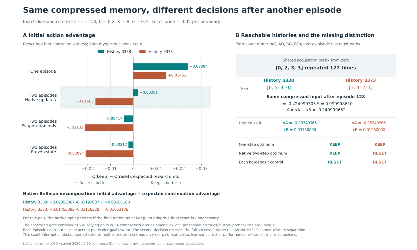
A small two-episode problem has twenty-seven thousand two hundred and twenty-five reachable states. Enumerating every one turned up two hundred and sixteen pairs that share a compressed summary and agree on the best immediate move, yet require opposite first moves once a second episode is in view. Without reinforcement the pairs agree. With it they split.
Then the more interesting question: was the option to correct course later what made those pairs differ? A separately frozen analysis of the saved values answered no. Every one of the two hundred and sixteen still split when the final move was forced to be the same. Six individual decisions changed when later observation was allowed, and none of them met the criterion.
What changed
The numerical line stopped there, at its declared scope. Widening the search until the more appealing explanation became true would not have answered the question that had already been asked.
| Initial decision | History A | History B |
|---|---|---|
| Best for one episode | Keep | Keep |
| Best over two episodes with reinforcement | Keep | Reset |
| Best over two episodes under either control without new reinforcement | Reset | Reset |
History A is 3338; history B is 3373 in the original figure. This table restates that pair. The reset price is 0.05 on a scale where each episode pays the expected fraction of routes that reach the goal, and the reference is given the full next state before its second choice at no charge.
Examine the original technical figure
08Arriving is not understanding
The hypothesis
A small transformer trained to walk these graphs would have to represent something like the endpoint field in order to route well. The field could then be found inside it.
What happened
Two models were trained. Both reached the requested ending on almost every attempt: 97.5 and 94.6 per cent. Both failed the routing test outright. With mean errors of 0.1421 and 0.1368 against an unguided baseline of 0.1214, they routed worse than no guidance at all.
The explanation came from an analytic check rather than the models. Under the task as it was posed, a policy that copies the requested ending and consults the legal-move mask, while ignoring every weight in the graph, reaches 97.73 per cent. The success rate was never evidence about the field. A paired audit across five hundred and twelve prompts confirmed it: the response to changing the goal was about a hundred-thousandth of what an oracle would show.
The task was then rebuilt as a direct local selection with the shortcut removed, and it has run three times since, each with its pass threshold fixed before the data existed. On the first run both models missed the threshold, and their error landed above even the best query-blind guess. A retrospective reading of the saved outputs found the missing contrast between paired queries to be the larger error in almost every pair. The second run turned on the output format. With fixed answer slots the model stayed accurate when the header was reversed, while with alias tokens it passed the original orientation and failed the held-out reversal in both seeds. On the third, teaching that reversal on half of the familiar pairs carried to the untaught half in all four folds. The fifty-six pairs that had never been legal sit at distances the model had never seen. Taken together they failed the acquisition threshold in every fold, and their error fell by a similar small amount in both orientations. So the result cannot tell pair-specific learning apart from an unfamiliar range that is simply harder.
What changed
No probe was run and no activation was patched, because there was nothing yet worth probing. The rebuilt task shows a learned finite local selector that transfers inside what it already knows. That is not a graph routing ability. The four folds share their controls, so they are not four independent replications. All six of the interpretability predictions remain untested, and that is the current state of the work.
04
Engineering
A world small enough to solve.
A record that can be audited.
Methods and checks
The search and decoding results on this page were measured inside a world small enough to solve completely, so each method could be scored against the exact answer. The rest of the engineering keeps that comparison fair and, since the provenance layer was added, ties each run’s numbers to the exact code and data that produced them.
- Ground truth
layered DAG 6 × 8, out-degree 3 · softmax over N(0,1) logits · trap_strength 1.5 · backward DP h(v) · logaddexp posterior, 1e-9 check · NumPy only
On a seeded random graph, the chance of reaching the goal from every state is solved backwards, from one at the goal and zero at the dead ends.
How it works
A seeded random graph of six layers, eight states wide, with three choices at every fork, built with NumPy alone. Each choice’s base probability is a softmax over random normal scores. Wherever the goal is still reachable but some children are dead ends, each dead-end edge has 1.5 added to its score, so the wrong turn is favoured on average. The chance of reaching the goal from every state is solved backwards, from one at the goal and zero at the dead ends. A forward pass gives the chance of each ending, and a law test pins the two passes as the same measure. On graphs small enough to enumerate (243 paths at these settings), every goal-reaching path is summed in log space and asserted equal to the backward answer within 1e-9.
- Decoding
P ∝ P0^(1/T) · ĥ^γ · e^(c·C) · Doob h-transform · K = 8 leader-streamer · conductance +0.6, decay 0.98 · T clipped to 0.25–3.0
One score serves every method: the base preference at temperature T, the estimated goal field raised to γ, and route credit C with gain c, so the comparisons switch one term at a time.
How it works
With T = 1, γ = 1, c = 0 and the exact field it is the Doob h-transform, exact sampling conditioned on reaching the goal, which is prior art the project concedes. The ensemble runs eight walkers and sets its temperature from how spread out they are and how concentrated the field is at their tips, held between 0.25 and 3.0. It deposits 0.6 of route credit (the conductance) on every edge of a circuit it believes succeeded, and decays all credit by 0.98 each episode.
- Fair comparison
compute-matched in transitions · K per layer step · oracle-free reinforcement · ĥ(tip) ≥ 0.5 × max terminal ĥ · truth stamped as measurement
One sampled edge costs one unit and the eight-walker ensemble pays eight per step, so under the same budget it gets about an eighth as many episodes, a ratio a law test holds within 2%.
How it works
The controller does not read the true goal. It reinforces only circuits whose tip its own field rates at least half as likely as its best ending and commits to the tip with the highest estimated field. The true outcome is stamped on the record afterwards. An earlier version did consult the goal. Hostile review found that, and it was removed before the decoy study was run. That study needed a controller able to lock onto a wrong channel.
- Measured
success per episode · transitions to first success · dead-end mass · KL from the exact posterior · seed bootstrap, 10,000 resamples · 40 seeds × 34 cells, 1,360 of 1,360
Four metrics let success be contradicted, measuring success per episode, transitions to a first success, the share of episodes that reach a dead end, and divergence from the exact posterior.
How it works
Four metrics, chosen so that success can be contradicted: success per episode, sampled transitions to a first success, the share of episodes that enter a state with no route to the goal, and the divergence of the sampled successful routes from the exact posterior. On these graphs the dead-end share is the complement of success, kept to show where the failures went. The wrong-channel rate in the decoy episode, twelve of thirty-one, carries a percentile interval from ten thousand seed-bootstrap resamples, and every one of the reanalysis’s 1,360 seed-by-condition cells completed.
- Model arm
111,400-parameter pre-LN causal transformer · 2 blocks · width 64 · 4 heads · FFN 256 · soft-target distillation from exact DP · isomorphism-keyed splits 256 / 64 / 128 · pinned lock, torch 2.7.0+cpu · monitored CPU phases, RSS cap 1.5 GiB
A transformer small enough to train on a CPU learns from the exact next-choice distributions of the backward solve, with graph-illegal moves masked.
How it works
The transformer is small enough to train and check on a CPU, and it learns from soft targets that are the exact next-choice distributions from the backward solve, with graph-illegal moves masked. The 256 training, 64 calibration and 128 test graph classes are separated by a layer-preserving isomorphism key, so a relabelled copy of one graph cannot cross splits. The latest runners will not start unless Python, torch and every installed package match a ten-package lock. Each phase runs as a monitored child process, stopped if its memory passes 1.5 GiB or a poll gap passes one second.
- Provenance
manifest before any work · git HEAD + porcelain status · SHA-256 of inputs and outputs · source byte snapshots · exclusive-create, atomic replace
Since the provenance layer was added, a run reserves a fresh directory (an existing one is refused) and writes its manifest before any work.
How it works
The manifest records the git state, the exact command, the interpreter and platform, every installed distribution, hashes of the inputs and byte copies of the source files it loads. The run also checks that those modules resolve to the intended checkout. Outputs are created exclusively, so nothing is overwritten. The manifest is replaced atomically and writes after completion are rejected. Before a run is marked complete, finalize re-hashes the inputs and every output. An interrupted run keeps a manifest marked incomplete.
- Verification
designs frozen before data · gates fixed in advance: mean TV ≤ 0.025, p95 ≤ 0.05 · separate data and result auditors · parity checks before training · 49 test files, 555 test functions · 16 law tests
A design and its code are committed before any data exists, findings cite that commit, and an analysis added afterwards is labelled retrospective.
How it works
Pass thresholds are fixed before the run (for the rebuilt task, a mean total variation from the exact answer of at most 0.025, and at most 0.05 at the 95th percentile) and a miss is published as a result. The first run of that task failed its gate and is recorded as a registered negative. Since the model arm began, separate audit scripts recompute the data and the results from saved outputs, and the three experiments on the rebuilt task carry six audits, all recorded as passed. The latest run replays archived outputs and applies an empty-exposure sham update before any training, and its design stops the run if either check differs. Its six fits ran to exactly 5,000 updates over 960,000 training presentations and 179,712 registered evaluation rows, with the parity checks counted separately. The test suite defines 555 functions across 49 files. Sixteen of them are law tests, pinning the Doob reduction, γ = 0 recovering the base process, the forward and backward passes agreeing, the compute-matched budget, and the belief gate matching the oracle gate under an honest field.
| Regime | Success per episode bar to 1 | KL from the exact posterior bar to 2 | First success after this many transitions |
|---|---|---|---|
| Fixed temperature | 0.025 | 0.309 | 824 |
| Goal-blind adaptive temperature | 0.032 | 0.289 | 507 |
| Exact field | 1.000 | 0.005 | 5 |
| Degraded field | 0.409 | 0.307 | 26 |
| Degraded field, ensemble and route credit | 0.999 | 1.979 | 44 |
Limits. The five-decoder figure is one configuration from the project’s first full run, made before the score form separated temperature from field strength and before the controller stopped consulting the goal. That run predates the provenance layer and has no manifest. The 555 is a count of defined test functions, and no passing run is claimed. The auditors are separate scripts and agents inside the project, so the audits are internal checks and nothing has been replicated outside it. The steering rule and the route credit are prior art, and what the project adds is the measurement layer around them. The interpretability arm, I1 to I6, has not run.
The current position
What the experiments
have established.
This is where the investigation currently stands. The correspondence table and prediction ledger distinguish what the tests support, what is partial, and what remains untested. They will keep changing as the research continues.
The mapping between lightning and generation
- 01Electrical potential fieldLearned landscape of preferences over continuationsscores at each stateMapped
- 02The descending stepped leaderA partial trajectory being sampleda path under the base processMapped
- 03Multiple leader tips branchingAn ensemble of candidate continuationsK partial paths, K = 8Mapped
- 04Ionisation lowering the breakdown thresholdRoute credit that decays unless renewedconductance, deposited and evaporatingMapped
- 05The upward streamer from the groundThe backward endpoint fieldh(s), and the transform that steers by itMapped
- 06Attachment: leader meets streamerCommitment to a goal-compatible regiona concentration event, not yet identifiedSpeculative
- 07The return strokeCredit assigned along the completed routereinforcement on the winning pathMapped
- 08Breakdown probability against field strengthStrength of endpoint guidancefield exponent γ, distinct from base temperatureMapped
- 09One channel versus manySearching versus samplingconditioning spreads; memory and cooling collapseMapped
- 10Charge accumulating in the cloudConstraint building up before generation startsnone written down yetSpeculative
- 11Restrikes down the same channelReusing a route that already workedcredit persisting across episodesTestbed only
- 12Breakdown that prefers a directionDifferent temperatures for settled and unsettled choicesa directional temperature, no observable yetSpeculative
- 13Laplace’s equation governs how a channel growsSteering by the endpoint field is a harmonic problemthe same boundary-value schemaMapped
- 14Forward sweeps and reverse replay in the brainSweeping over futures; assigning credit backwardsan adjacent field, nothing tested hereSpeculative
- 15A strike to the tallest wrong objectConfident commitment to a wrong endinga field wrong about the ending, measuredMapped
10 with an equation and a prediction4 still generating hypotheses1 proven in a testbed, unproven in a language model
No row here is marked falsified. The falsifications live one level down, in the predictions each row had to produce.
The predictions and their verdicts
| Id | What was predicted | What it earned |
|---|---|---|
| D1 | Temperature alone trades diversity without systematically improving success | Confirmed |
| D2 | Exact guidance is exact conditioning: success one, and the walk never enters a dead region | Confirmed |
| D3 | A degraded field degrades gracefully, between the baseline and the exact case | Confirmed at one setting |
| D4 | Composition recovers what a degraded field loses, at matched compute | Confirmed; endpoints corrected |
| D5 | Commitment is a sharp event rather than a drift | Instrument failed |
| D6 | Search-tree geometry interpolates with temperature as breakdown geometry does with the exponent | Untested |
| D7 | A wrong field produces confident, stable, false convergence, and confidence diverges from correctness | Mixed; disconfirmed on the strict reading |
| I1–I6 | The interpretability arm: a readable field inside a trained model, a commitment event, a causal intervention that switches the route | Untested, all six |
Instrument failure and falsification are recorded as different outcomes, and a failed entry stays in the table rather than being removed. A mapping that breaks is a boundary found, which is knowledge. Negative space is the most expensive ink on this map.
What this research cannot yet tell us.
Coherence is not truth
The mechanism produces agreement with whatever field it is given. A wrong field yields confident, stable, false convergence, both in the decoder and in the people reading its output. The rule applies reflexively: demote entries eagerly, and treat elegance as a prior rather than as evidence.
A beautiful correspondence is not a licence
New entries entering the mapping table arrive as speculative, with the missing piece named as either a formal object or something measurable. None skips that gate for being pleasing.
Published tokens cannot be recalled
A leader tip can stall harmlessly; an emitted token cannot be taken back. Anything that genuinely works like a leader needs reversible latent branches. The published stream belongs to the return stroke, not the leader.
Why keep asking?
What I learned
from the tests.
What has been established is narrow and worth stating plainly. Exact steering behaves exactly as its established mathematics requires. A field wrong about the ending produces confident wrong commitment in a constructed graph, and confidence measured from inside carries no information about it. Compressed memory can be insufficient in ways that are provable rather than arguable. Nothing here demonstrates a mechanism inside a trained transformer, and the lightning-like commitment event has not been shown to exist.
The value of this continuing project, for me, is making a speculative idea precise enough that evidence can change it. Every number above was allowed to revise the story that produced it, and several did. The next questions have to specify what information is available, which future actions are permitted, and what counts as a useful outcome. I’ll keep returning to the hypotheses, testing them and adding what those experiments reveal.
I supplied the original question and set the direction. ChatGPT helped develop the initial framing; Codex and Claude contributed the mathematical reductions, the code, the experiments and the critical review, under a working agreement that let the investigation retire its own hypotheses. Separate agents reconstructed calculations and checked claims against saved evidence. Those were internal verification steps, not external scientific replication.
Research log
The research log, newest first.
19 entries since 11 Jul 2026, the latest on 26 Sep 2026. From Lichtenberg experiment ledger (private research repository).
Reversal training carries to familiar pairs only
Teaching the small model to handle reversed order on half of its familiar option pairs carried over to the other half in all four runs, and in none of the four to pairs it had not seen as options.
- Limit It shows a bounded training effect on one task and does not establish a general rule or an internal pointer. The miss on new pairs may reflect their difficulty.
Output format decides whether a learned choice survives reordering
Every version learned the task in its trained order. When the two options were listed in reverse, answers given in fixed positions stayed accurate, while answers written as option labels fell short of the accuracy bar, though they partly adapted.
- Limit It is a result about what the task demands, and it leaves open both the internal mechanism and whether reversal can be learned in general.
The small model could not pick the asked-for row at this budget
Asked to select one of two displayed probability rows, the unchanged small network missed the target in every run, reacting about equally to the row it was asked about and the one it was not.
- Limit The result holds for this model, task and training budget, and does not show the design is incapable of it.
The trained models did not follow the local route weights
Rereading the saved predictions, the two models' choices sat further from each graph's actual route weights than a uniform guess would.
- Limit It is a look back at results already seen, with no new model runs, and identifies no internal mechanism.
Earlier entries (15)
The trained models barely respond when the goal changes
Across 512 paired prompts, swapping the requested goal shifted the models' route choices by about a hundred-thousandth of what an exact reference shifts, and their routing stayed slightly worse than uniform.
- Limit The tiny responses that remain do not show useful goal use, and cannot say whether they are noise or come from any internal mechanism.
A shortcut that could produce high success, and a test to expose it
Analysis showed that copying the requested ending and following the list of legal moves reaches 97.73 percent success while ignoring the graph's route weights, and a paired audit was designed around that shortcut.
- Limit Designed and not yet run. The shortcut is a worked control on reduced models, and it was not fitted to the trained ones.
Two small models reach the goal but do not route by it
Two small neural networks trained on the graphs reached the requested ending with 97.5 and 94.6 percent success, computed exactly over every graph and goal tested, yet their route choices were further from the ideal than unguided walking.
- Limit Reaching the goal often does not show the models learned goal-guided routes, and interpretation was deferred.
Designing the first trained-model test
A bounded test of whether a small neural network trained on these graphs learns to steer toward a requested goal was designed, and a separate check with no training showed its passes stay within an ordinary processor's limits.
- Limit Nothing was trained, so no model had learned anything yet, and all six predictions about internal mechanisms remained untested.
The option to change course later does not explain the split
Rechecking the saved values, all 216 pairs still called for different first moves when the final move was forced to be the same, so a later chance to revise does not explain the difference.
- Limit It holds for one problem family, horizon and reset price. Six single decisions changed when the next state could be seen, but that did not pass the controlled test.
When a memory summary is not enough over two episodes
Across all 27,225 reachable states of a small two-episode problem, 216 pairs share a compressed summary and the same best single move yet need opposite first moves once reinforcement carries into a second episode.
- Limit These histories were prescribed, so they say nothing about how often this happens.
Bounding what a compressed memory can know
An exact calculation of the range of goal chances consistent with a compressed memory settled the right action in 508 of 512 cases at one set of prices.
- Limit It uses one fixed price profile on one graph and supports no claim about average efficiency or the general value of extra information.
Recovery from a wrong ending when route memory is kept
On a small diamond-shaped graph, searches that first learned the wrong ending recovered in 231 of 256 runs when their route memory was kept, against 255 of 256 when the preference for that ending was erased.
- Limit It covers one small graph with fixed settings, and which intervention looks best depends on how recovery is measured.
Trying to reproduce a dropped value, without success
Sixty-four fresh language-model calls that varied the suspected causes produced no omissions, and all 256 retained values were correct.
- Limit Every task returned to its starting state, so copying the input would also score perfectly, and the earlier failure stays unexplained.
A model keeping a running record, with and without an archive
Over 48 language-model sessions every answer the record supported came back correct, but both conditions dropped the same known earlier value on identical input, and access to an archive repaired it at the next step.
- Limit It is one failure pattern on one pair of identical inputs, and gives no error rate.
A language model pulling records out of a history
Extracting records from 11 fixed histories, a language model reached the 55 percent ceiling that a two-record lookup allows under both prompts, so the added guidance showed no gain.
- Limit The task hit its ceiling, so it cannot show whether guidance helps, and it shows narrow model behavior, with no mechanism identified.
Pricing what a search should remember
An exact cost model comparing 20 fixed policies over 160 traces showed the cheapest one depends on the prices assumed: look information up when an archive is cheap, keep it when the archive is expensive.
- Limit The costs are declared assumptions, and nothing here tests a learned summary or a neural network.
How quickly a search recovers from memory built on a wrong answer
As reinforcement grew stronger, searches whose route memory started on the wrong answer recovered in 247, then 59, 3 and 0 of 256 runs. A sharp final answer appeared even without memory, so sharpness alone does not show memory at work.
- Limit It covers this exact model only, and did not test for a sudden tipping point or for trained networks.
Correcting the first graph results
Rereading the saved runs showed the combined system held on to a found route far more reliably than the comparison with a degraded guide (0.999 against 0.409) but found it more slowly, so the claim of faster discovery was withdrawn.
- Limit No new experiment was run, and those numbers came from an early controller that used the true goal to decide what to reinforce, changed before wrong goals were tested.
First graph runs: steering toward a goal, and how it goes wrong
The first runs on one family of constructed graphs were summarized at the time as four predictions confirmed, one measuring instrument failed, and a mixed verdict on how a wrong goal signal leads the search astray.
- Limit That summary was later superseded: the faster-discovery prediction was unsupported, and the early controller had used the true goal when deciding what to reinforce.